6 minute read · Ultimo Research Desk · Reviewed 5 Sept 2026
Trend Following: What It Is, What It Requires and Where It Fails
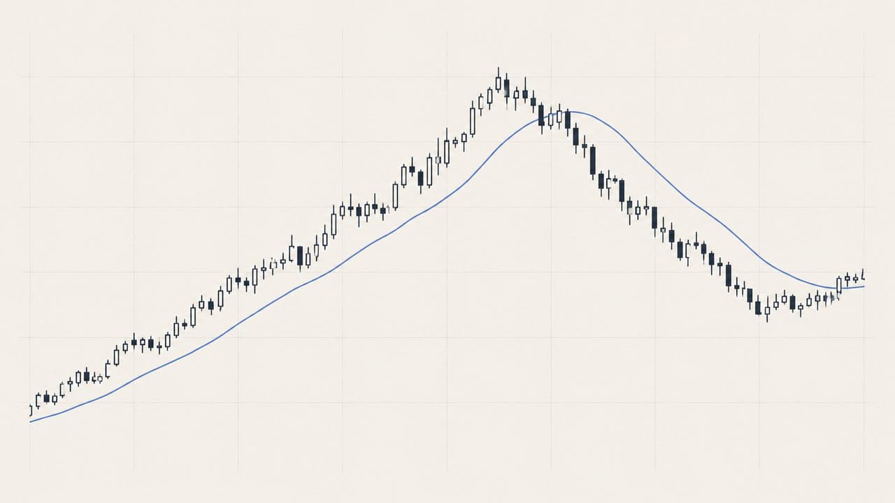
Trend following is an approach that keeps exposure aligned with a sustained price direction and reduces or reverses that exposure when the direction changes. It depends most on directional persistence lasting long enough to cover delayed signals, losing trades and dealing costs.
What it is
Trend following treats price direction as information about the current market state. It does not require a view about fair value. A trend-following model may compare prices with a moving average, identify a new high or low in a rolling channel, or measure the direction of a longer price series. The common feature is that the model responds to movement that has already appeared. It does not attempt to forecast every short-term fluctuation.
The approach is used across equity indices, individual shares, foreign exchange, interest-rate instruments, commodities and other liquid markets. Timeframes range from several days to several months. A short look-back reacts earlier but changes direction more often. A long look-back reacts later and can remain exposed after a move has weakened. Trend following is a family of rules, not one standard formula, and has no single inventor. Donchian’s channel work and the time-series momentum literature are documented parts of its development.
A trend can be defined separately for each instrument, or a portfolio can compare recent returns across instruments. Cross-sectional momentum ranks instruments against one another; time-series momentum compares an instrument with its own past direction.
What it requires
Trend following usually requires less continuous screen time than intraday approaches, but it requires regular monitoring of open positions, signals, cash and market closures. A model that operates on daily data can be checked at a scheduled time, while one that uses intraday data needs more reliable data and more frequent decisions. The required attention is therefore determined by the shortest decision interval, not by the name of the approach.
Capital must be sufficient for a series of small losing trades and for gaps through a planned exit level. Position size is often linked to estimated volatility so that a high-volatility instrument does not dominate the portfolio simply because its price moves more. That makes the capital requirement depend on the number of instruments, the intended holding period and the tolerance for interim drawdown. A small account can calculate the signal, but limited capital can prevent meaningful diversification.
The approach is easier to implement in instruments with dependable historical prices, regular trading hours or clearly defined sessions and sufficient liquidity. Data must be adjusted consistently for splits, contract rolls and other discontinuities. Execution quality matters most when the signal changes after a fast move, at a market open or after a weekend gap.
How it is implemented
An implementation first defines the data interval and the price used in the calculation. It then defines a directional reference, such as a moving-average relationship, a channel boundary or a price change over a specified look-back. A position is opened or increased when the reference indicates a direction and reduced, closed or reversed when a separate exit condition changes that indication. The precise rule, timing and treatment of equal values must be fixed before testing.
Position sizing is commonly based on a fixed fraction of available capital, a volatility estimate, or a risk amount between the entry and the model’s exit level. A portfolio may cap exposure to correlated instruments. Financing, contract rolls, dividends and currency conversion must be included in the accounting. A trailing exit can protect part of a move but can close during a temporary retracement.
Worked example
Assume one unit, a signal to hold a long position, a mid-price entry of 100 and a mid-price exit rule. The quoted spread is assumed to be 0.10 at each trade, so the round-trip spread cost is 0.10. Commission is assumed to be 0.20 on entry and 0.20 on exit. Financing is assumed to be 0.05 per day for three days, or 3 × 0.05 = 0.15. Total assumed cost is therefore 0.10 + 0.20 + 0.20 + 0.15 = 0.65.
In a winning case, the exit mid-price is 103. The long position’s gross price result is 103 − 100 = 3.00. Net result is 3.00 − 0.65 = 2.35 price units.
In a losing case, the exit mid-price is 98. The gross price result is 98 − 100 = −2.00. Net result is −2.00 − 0.65 = −2.65 price units. The figures are illustrative assumptions. They show that the same direction rule has to absorb costs in both outcomes and that the losing outcome is not removed by a trend reference.
Costs
Spread and commission are paid whenever a signal changes the position. A long holding period can make those costs smaller relative to the gross price movement, but a slow or sideways market can create repeated signals without a large movement to offset them. Slippage tends to increase when a signal arrives after a gap, during a fast reversal or in a thin market.
Financing applies when a position is held beyond the relevant daily cut-off, and contract-based instruments can incur roll effects. A portfolio that holds several markets also carries currency conversion and collateral costs. A volatility-based position-sizing method does not make those costs disappear; it changes the number of units held. Historical testing that omits dealing costs, funding and realistic fills can materially misstate the approach.
Where it fails
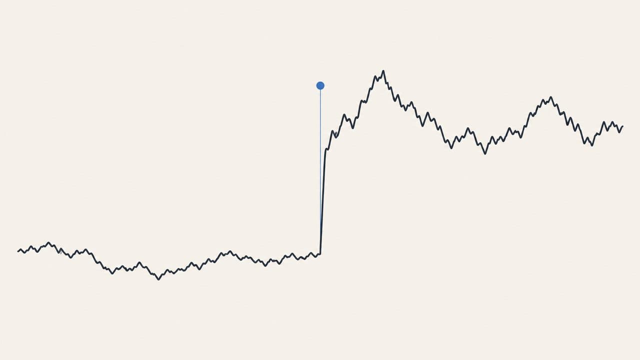
Trend following is hurt by a range with repeated reversals. The model can enter after a move begins, be closed when the move pauses, and then enter again when the range breaks in the opposite direction. Several such trades can occur before a sustained move appears. A sudden reversal can also turn a previously favourable position into a loss before a daily signal updates.
The approach can fail when the chosen reference is fitted to one market or historical period. A look-back can be too fast in a range or too slow after a regime change. Correlated instruments can express the same underlying shock. Behavioural errors include cancelling a model after losses, increasing size after a win or changing the exit after the signal has been generated.
Who it suits and who it does not
Trend following is more compatible with a reader who can review positions at a defined interval, accept delayed entries and tolerate a sequence of losing trades without changing the rules. It also requires enough capital for sensible position sizing and for positions to remain open through ordinary volatility.
It is less compatible with someone who needs frequent decisions, cannot monitor overnight or weekend risk, or cannot tolerate a model that may give back part of an earlier move. It is also unsuitable for a portfolio where the intended holding period is shorter than the data and execution process can support.
What the evidence says
Moskowitz, Ooi and Pedersen (2012) examined time-series momentum in 58 liquid futures instruments across equity indices, currencies, commodities and bonds. They reported persistence over horizons from one to twelve months, followed by partial reversal at longer horizons. That evidence concerns a specified research design, futures data and historical implementation costs. It does not establish that every trend-following rule, market or retail implementation has the same behaviour.
Jegadeesh and Titman (1993) documented medium-term continuation in a cross-sectional stock-ranking setting. That is related to momentum but is not identical to following each instrument’s own trend. Park and Irwin (2007) reviewed technical-rule research and identified mixed evidence and recurring problems involving data selection, changing market conditions and costs. The literature therefore supports treating trend following as a testable family of rules with exposure to particular regimes, not as a general conclusion about future price direction.
Sources
- Moskowitz, Ooi and Pedersen (2012), “Time Series Momentum”, DOI.
- Jegadeesh and Titman (1993), “Returns to Buying Winners and Selling Losers: Implications for Stock Market Efficiency”, DOI.
- Park and Irwin (2007), “What Do We Know About the Profitability of Technical Analysis?”, DOI.
- Sullivan, Timmermann and White (1999), “Data-Snooping, Technical Trading Rule Performance, and the Bootstrap”, DOI.
- John J. Murphy, Technical Analysis of the Financial Markets (1999), Google Books.
Educational only: Trend following can incur repeated losses in ranges and can give back gains during abrupt reversals.
Written by the Ultimo Research Desk and checked against our own contract specifications and client agreement before publication; reviewed again when those change. Educational only — nothing here is a recommendation to trade. Spotted an error? Tell us.